Surface Mesh Segmentation

Author

Ilker O. Yaz

Figure 1: Elephant model with SDF values & Segmentation.

Introduction

Mesh segmentation is the process of partitioning a mesh into smaller and meaningful sub-meshes. The application domain is wide and includes, but is not limited to modeling, rigging, texturing, shape-retrieval, and deformation. A detailed survey on mesh segmentation techniques can be found in Shamir2008SegmentationSurvey.

This package provides an implementation of the algorithm presented in Shapira2008Consistent. It relies on the Shape Diameter Function (SDF) which provides an estimate of the local volume diameter for each facet of the mesh. Given SDF values, the segmentation algorithm first applies soft clustering on facets. These clusters are then refined using a graph-cut algorithm which also considers surface-based features such as dihedral-angle and concavity.

The API gives access to both the SDF computation and segmentation for a given triangulated mesh. That way an alternative implementation of the SDF can be directly plugged into the segmentation algorithm. Also same SDF values can be used multiple times as a parameter for the segmentation algorithm.

Since the mesh segmentation problem is ill-posed, we also evaluate results of our implementation by using data set and evaluation software provided by Chen2009SegmentationBenchmark, and provide detailed results at the end of the manual.

Overview of the Segmentation Process

The segmentation algorithm consists of three major parts: Shape Diameter Function (SDF), soft clustering, and graph-cut for hard clustering.

Shape Diameter Function

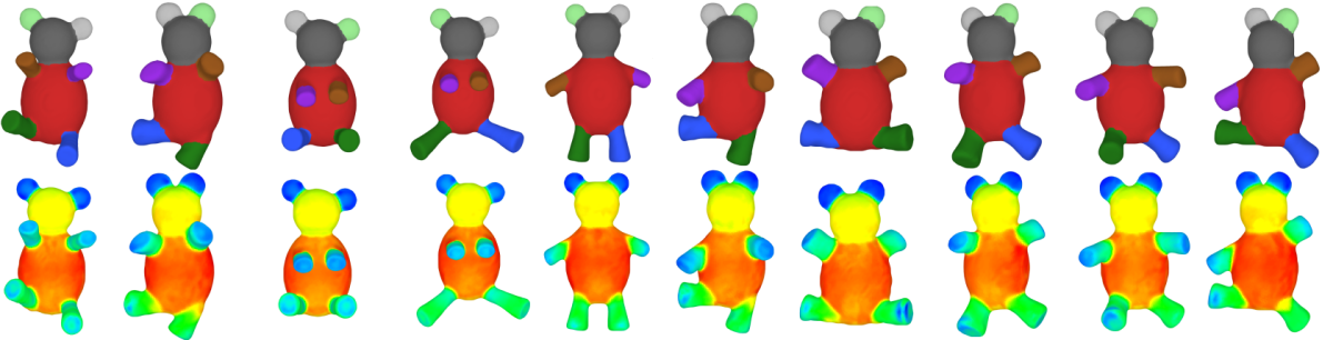
The Shape Diameter Function (SDF) provides a connection between the surface and its volume. More precisely, the SDF is a scalar-valued function defined on facets of the surface which measures the corresponding local volume diameter. The main handiness of the SDF is being able to distinguish thick and thin parts of the mesh by bringing in a volume-based feature to the surface. Another key feature of the SDF is its pose-invariant nature, which means that SDF values remain largely unaffected after changes of pose Figure-3.

The SDF over a surface is computed by processing each facets one by one. For a given facet, the SDF value computation begins with casting several rays sampled from a cone which is constructed using the centroid of the facet as apex and inward-normal of the facet as axis. Using these casted rays (which intuitively correspond to a local volume sampling), the SDF value is calculated by first applying outlier removal and then taking average of ray lengths.

Figure 2: Comparison of biased-to-center and uniform disk sampling for 64 rays.

We use sampling method from Vogel1979Sampling to sample points from base of the cone, then combine them with apex of the cone as origin while constructing rays. Our sampling method is biased to center in order to make sampling uniform to angle. As a result, we do not use mentioned weighting schema, stated in the paper, in order to reduce the contributions of rays with larger angles. A comparison with biased and uniform sampling of points can be seen in Figure-2. The final SDF value of a facet is then calculated by averaging the ray lengths which fall into one Median Absolute Deviation (MAD) from the median of all lengths.

After calculating SDF values for each facet, bilateral smoothing (an edge-preserving filtering technique) Tomasi1998Bilateral is applied. The purpose of edge-preserving smoothing is removing noise while keeping fast changes on SDF values in-place without smoothing, since they are natural candidates for segment boundaries. Window size \( w \), range parameter \( \sigma_r \), and spatial parameter \( \sigma_s \) are parameters for bilateral smoothing and determined as follows: windows size is set to \( w = \sqrt{number\:of\:facet / 2000} + 1 \), spatial parameter is half of the window size \( \sigma_s = w /2 \), range parameter is determined for each facet by computing standard deviation of SDF values around the SDF value of current facet \( \sigma_{r_i} = \sqrt{1/|w_i|\sum_{f_j \in w_i}(SDF(f_j) - SDF(f_i))^2} \).

Figure 3: Effect of pose changes on segmentation and SDF values.

Soft Clustering

The soft clustering on computed SDF values first groups facets using k-means clustering algorithm which is initialized with k-means++ (an algorithm for choosing random seeds for clusters) and run multiple times. Among these runs, we choose clustering result that has minimum with-in cluster error and use it to initialize expectation maximization algorithm for fitting Gaussian mixture models.

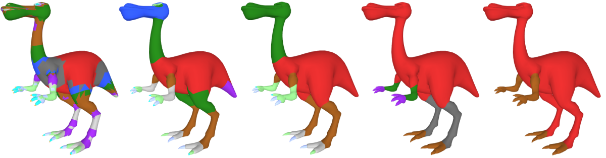
Note that there is no direct relationship between the number of clusters (parameter for soft clustering) and the number of segments (i.e. disconnected components / surface patches). Intuitively, the number of clusters represents the number of levels of a segmentation by clustering facets which have close SDF values without considering their connectivity. However, a large number of clusters is likely to result in detailed segmentation of the mesh with a large number of segments Figure-4.

The output of this step is a matrix that contains probability values for each facet to belong to each cluster. These probability values are used as input in the graph-cut step that follows.

Figure 4: Effect of different number of clusters on the segmentation. Number of clusters were set to 4, 3, and 2 respectively.

Graph-Cut

The final hard clustering, which gives the final partitioning of the mesh, is obtained by minimizing an energy function. This energy function combines the aforementioned probability matrix and geometric surface features. The result of the algorithm is assigned clusters for each facet, however we postprocess the result and produce a unique ID for each set of facets which are connected and placed under same cluster (i.e for each segments / surface patches).

The expression of energy function that is minimized using alpha-expansion graph cut algorithm Boykov2001FastApproximate is the following:

\( E(\bar{x}) = \sum\limits_{f \in F} e_1(f, x_f) + \lambda \sum\limits_{ \{f,g\} \in N} e_2(x_f, x_g) \) \( e_1(f, x_f) = -log(max(P(f|x_f), \epsilon)) \) \( e_2(x_f, x_g) = \left \{ \begin{array}{rl} -log(\theta(f,g)/\pi) &\mbox{ $x_f \ne x_g$} \\ 0 &\mbox{ $x_f = x_g$} \end{array} \right \} \)

where: \(F\) is the set of facets, \(N\) is the set of pairs of neighbor facets, \(x_f\) is the cluster assigned to facet \(f\), \(P(f|x_p)\) is the probability of assigning facet \(f\) to cluster \(x_p\), \(\theta(f,g)\) is the dihedral angle between neighbor facets \(f\), and \(g\), concave angles and convex angles are weighted by 1 and 0.1 respectively, \(\epsilon\) is the minimal probability threshold, \(\lambda \in [0,1]\) is a smoothness parameter.

The first term of the energy function provides the contribution of the soft clustering probabilities. The second term of the energy function is larger when two neighbor facets sharing a sharp and concave edge are in the same cluster. The smoothness parameter can be used to make this geometric criteria more or less prevalent.

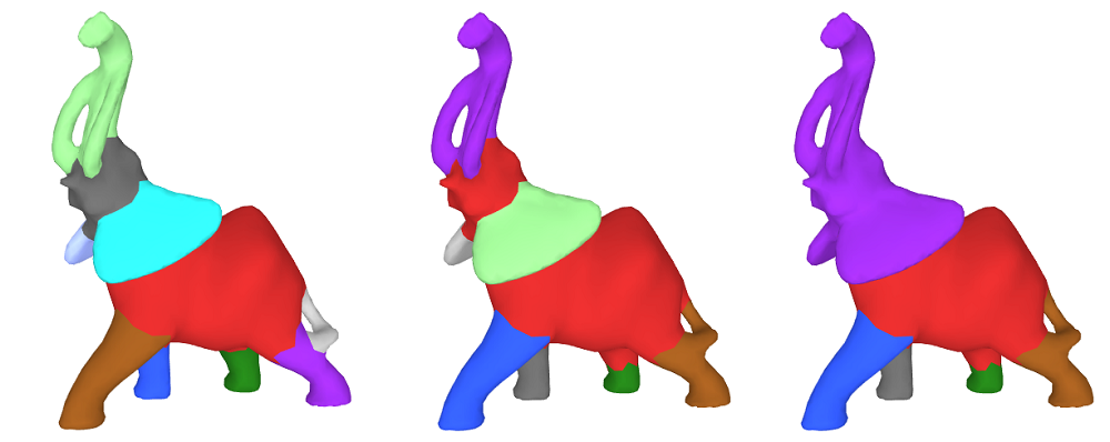
Basically, assigning a high value to smoothness parameter results in small number of segments since constructing a segment boundary would be expensive. Another words, merging facets which are placed under different clusters is less expensive than separating them and creating boundaries. Similarly, assigning smaller values to smoothness parameter results in high number of segments by getting closer to the result of soft clustering (notice that setting smoothness parameter to zero directly returns the result of soft clustering). Effect of different smoothness parameters is demonstrated in Figure-5.

Figure 5: Effect of different smoothness parameters on the segmentation (10 clusters). The smoothness parameter was set to 0.0, 0.1, 0.25, 0.5 and 1.0 respectively.

API

This package provides three functions:

• CGAL::compute_sdf_values : computes SDF values as described in the original paper.
• CGAL::segment_from_sdf_values : computes the mesh segmentation from SDF values.
• CGAL::compute_sdf_values_and_segment : computes SDF values and mesh segmentation in one go (i.e. combines two functions listed above).

These functions expects a manifold, normal oriented, and triangulated polyhedron without boundary as input. Note that the current implementation is working with polyhedron with boundaries, but considering how the SDF value are computed, using a polyhedron with large holes is likely to result in meaningless SDF values, and therefore unreliable segmentation.

The current implementation of the computation of the SDF values relies on the AABB_tree package. This operation is reliable when the AABBTraits model provided has exact predicates.

The SDF Computation

The function CGAL::compute_sdf_values provides an implementation of the SDF computation for a given CGAL Polyhedron.

After computation, the following post-processing steps are applied:

• Facets with no SDF values (i.e. zero) are assigned to average SDF value of its neighbors. If still there is any facet which has no SDF value, minimum SDF value greater than zero is assigned to it. Note that this step is not inherited from the paper.
• Smoothed with bilateral filtering.
• Linearly normalized between [0,1].

The outputs are a property map which associates every facet with its SDF value, and pair of minimum and maximum SDF values before linear normalization.

Example

#include <CGAL/Exact_predicates_inexact_constructions_kernel.h>
#include <CGAL/Polyhedron_3.h>
#include <CGAL/IO/Polyhedron_iostream.h>
#include <CGAL/mesh_segmentation.h>

#include <boost/property_map/property_map.hpp>

#include <iostream>
#include <fstream>

typedef CGAL::Exact_predicates_inexact_constructions_kernel Kernel;
typedef CGAL::Polyhedron_3<Kernel> Polyhedron;

int main(int argc, char **argv)
{
    if (argc !=2){
        std::cerr << "Usage: " << argv[0] << " input.off" << std::endl;
        return 1;
    }
  
    // create and read Polyhedron
    Polyhedron mesh;
    std::ifstream input(argv[1]);
    
    if ( !input || !(input >> mesh) || mesh.empty() ){
        std::cerr << argv[1] << " is not a valid off file." << std::endl;
        return 1;
    }
        
    const int number_of_rays = 20;                   // cast 30 rays per facet
    const double cone_angle = (1.0 / 2.0) * CGAL_PI; // use 90 degrees for cone opening-angle

    // create a property-map
        typedef std::map<Polyhedron::Facet_const_handle, double> Facet_double_map;
    Facet_double_map internal_map;
    boost::associative_property_map<Facet_double_map> sdf_property_map(internal_map);

    // use custom parameters for number of rays, and cone angle.
    std::pair<double, double> min_max_sdf = CGAL::compute_sdf_values(mesh, sdf_property_map, cone_angle, number_of_rays);
        // for using default parameters: CGAL::compute_sdf_values(mesh, sdf_property_map);
        
        // print minimum & maximum sdf values
    std::cout << "minimum sdf: " << min_max_sdf.first << " maximum sdf: " << min_max_sdf.second << std::endl;
        
    // print sdf values 
    for(Polyhedron::Facet_const_iterator facet_it = mesh.facets_begin(); 
        facet_it != mesh.facets_end(); ++facet_it)   
    {
        std::cout << sdf_property_map[facet_it] << std::endl;                                 
    }
}

Surface Mesh Segmentation

The function CGAL::segment_from_sdf_values computes a segmentation of the mesh using provided SDF values. Note that these SDF values can be any set of scalar value associated with each facet as long as they are linearly normalized between [0, 1]. This function also gives opportunity to use same SDF values multiple times with different parameters in segmentation stage.

The outputs are number of segments and a property map which associates a segment-id (an integer between [0, number of segments -1]) to each facet. Formally, a segment is a set of connected facets which are placed under same cluster after graph-cut. Note that the number of clusters, which is the input parameter of the algorithm, and the number of partitions in the final segmentation (the actual output of the algorithm) are not equal.

Example

#include <CGAL/Exact_predicates_inexact_constructions_kernel.h>
#include <CGAL/Polyhedron_3.h>
#include <CGAL/IO/Polyhedron_iostream.h>
#include <CGAL/mesh_segmentation.h>

#include <boost/property_map/property_map.hpp>

#include <iostream>
#include <fstream>

typedef CGAL::Exact_predicates_inexact_constructions_kernel Kernel;
typedef CGAL::Polyhedron_3<Kernel> Polyhedron;

int main(int argc, char **argv)
{
    if (argc !=2){
        std::cerr << "Usage: " << argv[0] << " input.OFF" << std::endl;
        return 1;
    }
  
    // create and read Polyhedron
    Polyhedron mesh;
    std::ifstream input(argv[1]);
    
    if ( !input || !(input >> mesh) || mesh.empty() ){
        std::cerr << argv[1] << " is not a valid off file." << std::endl;
        return 1;
    }

    // create a property-map for sdf values (it is an adaptor for this case) 
    typedef std::map<Polyhedron::Facet_const_handle, double> Facet_double_map;
    Facet_double_map internal_sdf_map;
    boost::associative_property_map<Facet_double_map> sdf_property_map(internal_sdf_map);
        
    // compute sdf values using default parameters for number of rays, and cone angle
    CGAL::compute_sdf_values(mesh, sdf_property_map);
        
    // create a property-map for segment-ids (it is an adaptor for this case)
    typedef std::map<Polyhedron::Facet_const_handle, int> Facet_int_map;
    Facet_int_map internal_segment_map;
    boost::associative_property_map<Facet_int_map> segment_property_map(internal_segment_map);
        
    // segment the mesh using default parameters for number of levels, and smoothing lambda     
    int number_of_segments = CGAL::segment_from_sdf_values(mesh, sdf_property_map, segment_property_map);
        
    std::cout << "Number of segments: " << number_of_segments << std::endl;
    // print segment-ids
    for(Polyhedron::Facet_const_iterator facet_it = mesh.facets_begin(); 
        facet_it != mesh.facets_end(); ++facet_it)   
    {
        // ids are between [0, number_of_segments -1]
        std::cout << segment_property_map[facet_it] << std::endl;                                 
    }

    const int number_of_levels = 4;       // use 4 clusters in soft clustering
    const double smoothing_lambda = 0.3;  // importance of surface features, between [0,1]

    // Note that we can use same sdf values (sdf_property_map) over and over again for segmentation.
    // This feature becomes important when we want to segment the mesh several times with different parameters.
    CGAL::segment_from_sdf_values(
        mesh, sdf_property_map, segment_property_map, number_of_levels, smoothing_lambda);
}

The function CGAL::compute_sdf_values_and_segment combines the two aforementioned functions. Note that for segmenting the mesh several times with different parameters (i.e. number of levels, and smoothing lambda), it is wise to first compute the SDF values using CGAL::compute_sdf_values. Then, computed SDF values can be used several times when calling CGAL::segment_from_sdf_values with different parameters (i.e. number of levels, and smoothing lambda).

Example

#include <CGAL/Exact_predicates_inexact_constructions_kernel.h>
#include <CGAL/Polyhedron_3.h>
#include <CGAL/IO/Polyhedron_iostream.h>
#include <CGAL/mesh_segmentation.h>

#include <boost/property_map/property_map.hpp>

#include <iostream>
#include <fstream>

typedef CGAL::Exact_predicates_inexact_constructions_kernel Kernel;
typedef CGAL::Polyhedron_3<Kernel> Polyhedron;

int main(int argc, char **argv)
{
    if (argc !=2){
        std::cerr << "Usage: " << argv[0] << " input.OFF" << std::endl;
        return 1;
    }
  
    // create and read Polyhedron
    Polyhedron mesh;
    std::ifstream input(argv[1]);
    
    if ( !input || !(input >> mesh) || mesh.empty() ){
        std::cerr << argv[1] << " is not a valid off file." << std::endl;
        return 1;
    }

    // create a property-map for segment-ids (it is an adaptor for this case)
    typedef std::map<Polyhedron::Facet_const_handle, int> Facet_int_map;
    Facet_int_map internal_segment_map;
    boost::associative_property_map<Facet_int_map> segment_property_map(internal_segment_map);
        
    // calculate SDF values and segment the mesh using default parameters.
    int number_of_segments = CGAL::compute_sdf_values_and_segment(mesh, segment_property_map);

    std::cout << "Number of segments: " << number_of_segments << std::endl;
        
    // print segment-ids
    for(Polyhedron::Facet_const_iterator facet_it = mesh.facets_begin(); 
        facet_it != mesh.facets_end(); ++facet_it)   
    {
        std::cout << segment_property_map[facet_it] << std::endl;                                 
    }
}

Using a polyhedron with an ID per facet

The previous examples use a std::map as property maps for storing the SDF values and the segmentation results. This example uses a polyhedron type with a facet type having an extra ID field together with a vector as underlying data structure in the property maps. The main advantage is to decrease the complexity of accessing associated data with facets from logarithmic to constant.

Example

#include <CGAL/Exact_predicates_inexact_constructions_kernel.h>
#include <CGAL/Polyhedron_3.h>
#include <CGAL/Polyhedron_items_with_id_3.h>
#include <CGAL/IO/Polyhedron_iostream.h>
#include <CGAL/mesh_segmentation.h>

#include <boost/property_map/property_map.hpp>

#include <iostream>
#include <fstream>

typedef CGAL::Exact_predicates_inexact_constructions_kernel Kernel;
typedef CGAL::Polyhedron_3<Kernel, CGAL::Polyhedron_items_with_id_3>  Polyhedron;

// Property map using the fact that each facet is assigned an integer
// to store associated information into a vector
template<class PolyhedronWithId, class ValueType>
struct Polyhedron_with_id_to_vector_property_map
    : public boost::put_get_helper<ValueType&,
             Polyhedron_with_id_to_vector_property_map<PolyhedronWithId, ValueType> >
{
public:
    typedef typename PolyhedronWithId::Facet_const_handle key_type;
    typedef ValueType value_type;
    typedef value_type& reference;
    typedef boost::lvalue_property_map_tag category;

    Polyhedron_with_id_to_vector_property_map() : internal_vector(NULL) { }
    Polyhedron_with_id_to_vector_property_map(std::vector<ValueType>* internal_vector)
         : internal_vector(internal_vector) { }
        
    reference operator[](key_type key) const { return (*internal_vector)[key->id()]; }
private:
    std::vector<ValueType>* internal_vector;
};

int main(int argc, char **argv)
{
    if (argc !=2){
                std::cerr << "Usage: " << argv[0] << " input.OFF" << std::endl;
                return 1;
    }
  
    // create and read Polyhedron
    Polyhedron mesh;
    std::ifstream input(argv[1]);
    
    if ( !input || !(input >> mesh) || mesh.empty() ){
        std::cerr << argv[1] << " is not a valid off file." << std::endl;
        return 1;
    }

    // assign id field for each facet   
    int facet_id = 0;
    for(Polyhedron::Facet_iterator facet_it = mesh.facets_begin(); 
        facet_it != mesh.facets_end(); ++facet_it, ++facet_id)
    {
        facet_it->id() = facet_id;
    }

    // create a property-map for sdf values
    std::vector<double> sdf_values(mesh.size_of_facets()); 
    Polyhedron_with_id_to_vector_property_map<Polyhedron, double> sdf_property_map(&sdf_values);

    CGAL::compute_sdf_values(mesh, sdf_property_map);
        
    // access sdf values (with constant-complexity) either via sdf_values or sdf_property_map
    for(Polyhedron::Facet_const_iterator facet_it = mesh.facets_begin(); 
        facet_it != mesh.facets_end(); ++facet_it)
    {
        std::cout << sdf_property_map[facet_it] << std::endl; // or segment_ids[facet_it->id()]
    }

    // create a property-map for segment-ids 
    std::vector<unsigned> segment_ids(mesh.size_of_facets()); 
    Polyhedron_with_id_to_vector_property_map<Polyhedron, unsigned> segment_property_map(&segment_ids);

    CGAL::segment_from_sdf_values(mesh, sdf_property_map, segment_property_map);

    // access segment-ids (with constant-complexity) either via segment_ids or segment_property_map
    for(Polyhedron::Facet_const_iterator facet_it = mesh.facets_begin(); 
        facet_it != mesh.facets_end(); ++facet_it)   
    {
        std::cout << segment_property_map[facet_it] << std::endl; // or segment_ids[facet_it->id()]                               
    }
}

Implementation history

The initial implementation of this package is the result of the work of the author during the 2012 season of the Google Summer of Code.